|
|
| |
|
|
Wave2D: Modeling Examples
In the sequel several example modeling scenarios are given that should demonstrate the functionality of the program "Wave2D". The special properties of this scenarios are highlighted on the left of the following table and one or more scaled down screenshots are given on the right. Click the scaled down screenshots for a full version.
| Properties |
Screenshot |
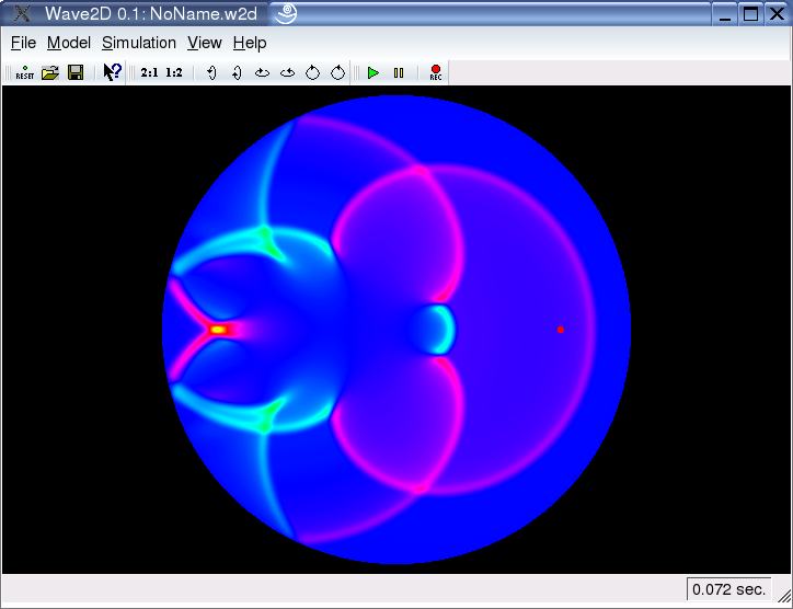
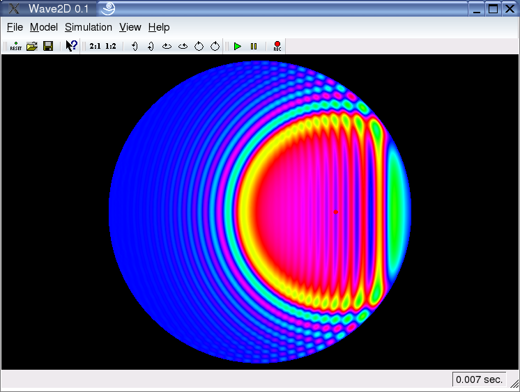
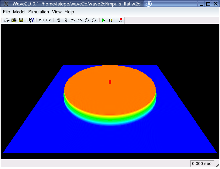
Excitation Signals:
To excite the wave field, "Wave2D" offers the possibility to define one or more excitation functions. Theses functions act uniformly distributed in a specific spatial region (see also the Spatial Excitations example) centered around the excitation point. The temporal behavior of these functions is arbitrary. One can either choose built in impulses (left screenshot), built in periodical functions (right screenshot) or even arbitrary functions from a wave-file.
The red marker on the screenshot indicates the excitation point and the green marker indicates an additional output point for sound recording.
|
|
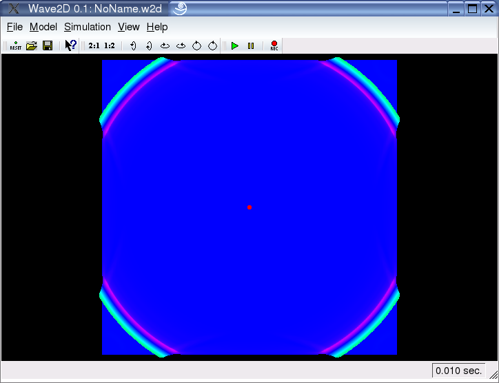
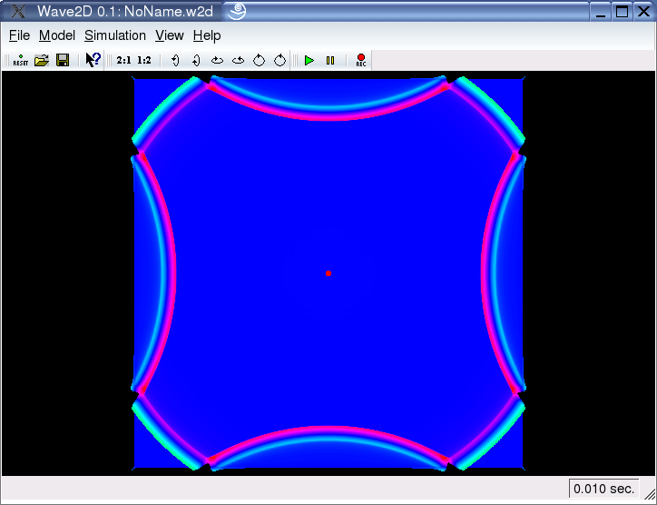
Boundaries:
Under certain limitations in the free-field scenario, it is possible to adjust the boundary conditions of an rectangular (triangular is in alpha stage) region continuous from full reflecting to absorbing (left screenshot). It is also possible to invert the reflections (see right screenshot), what would correspond to boundary conditions of zero deflection, as they are typical for supported membranes. Please note, that adjustable boundary conditions are so far not possible with circular regions.
|
|
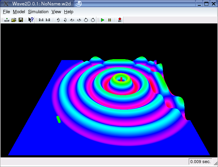
Drum Models:
Circular geometries play a special role in "Wave2D". In fact, circular models are membrane models. The visualized outcome is the deflection of this membrane, rather than the speed of the membrane (equivalent to pressure in room acoustics) as it is for rectangular models, and the boundary conditions are always supported for circular models compared to free boundary conditions for rectangular models. Together with the additional physical effects dispersion (resistance against bending) and frequency dependent and frequency independent damping, one can achieve a realistic drum model. The screenshots depict a simulation of the pure wave equation on the left (a thin membrane for instance), and a simulation of a strong dispersive material (a metal for instance) on the right.
|
|
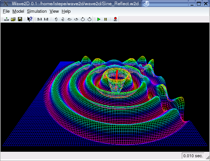
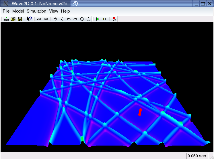
Spatial Grid:
For the visual representation of the wave field a spatial grid is required. There are several options concerning this grid. First of all, the resolution of this grid can be adjusted independently from the accuracy of the simulation. A low resolution will increase the speed of the simulation significantly, while the accuracy of the sound-output is unchanged.
The visual appearance of this grid can be either interpolated, as seen on the left screenshot, or as a wireframe graphics, as seen on the right screenshot. In the interpolate mode, the rectangles of the spatial grid are represented by two triangles. This might be visible for low grid resolutions.
|
|
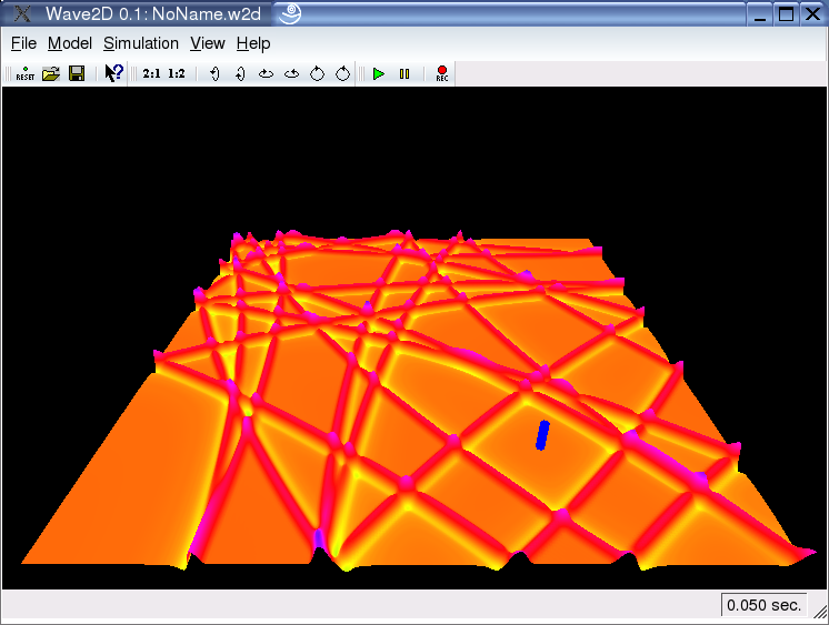
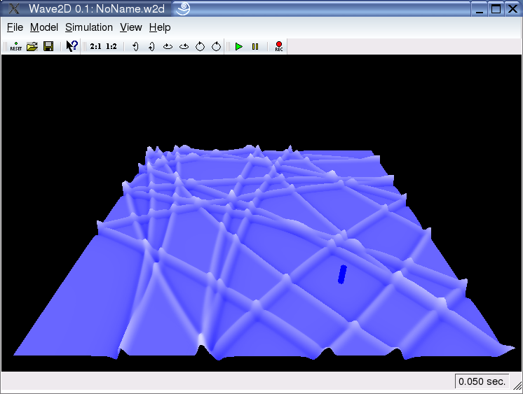
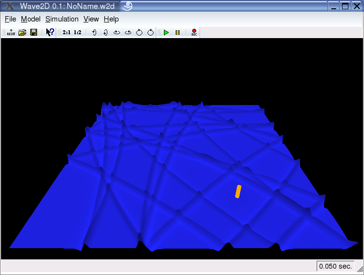
Colors:
"Wave2D" visualizes the amplitude of the 2D wave field by both, deflection in the third dimension and color. Concerning the color, the user can adjust a number of properties.
First of all, one can adjust all base colors, i.e. the color of the background, the input and output markers and the base color of the net, as it can be seen un the upper both screenshots.
Furthermore, one can define which color-property has to indicate the deflection. There are three possible options: color (both upper screenshots), saturation (lower left screenshot), and brightness (lower right screenshot).
|
|
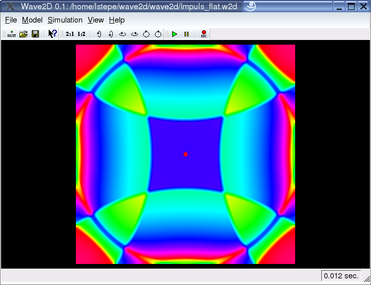
Spatial Excitations:
As already mentioned in the Excitation Signals example, each excitation function acts on a certain spatial region. The most simple region implemented is a single point, modeled with a spatial Dirac-function. However, for realistic excitation models is it also possible to excite a circular region around the excitation position. The user can adjust the radius of this region. Furthermore, one can choose between a "flat" excitation, where all points within this circular region are equally excited (see screenshot on the left), or a "parabolic distribution, where the amount of excitation decreases with the radius.
Spatially distributed excitations can create nice effects. The screenshot on the right was taken a few milliseconds after the model was excited in a large region.
|
|
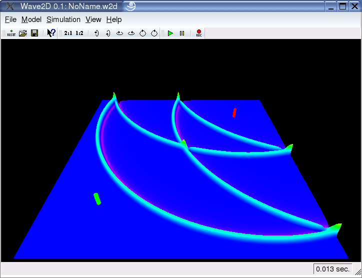
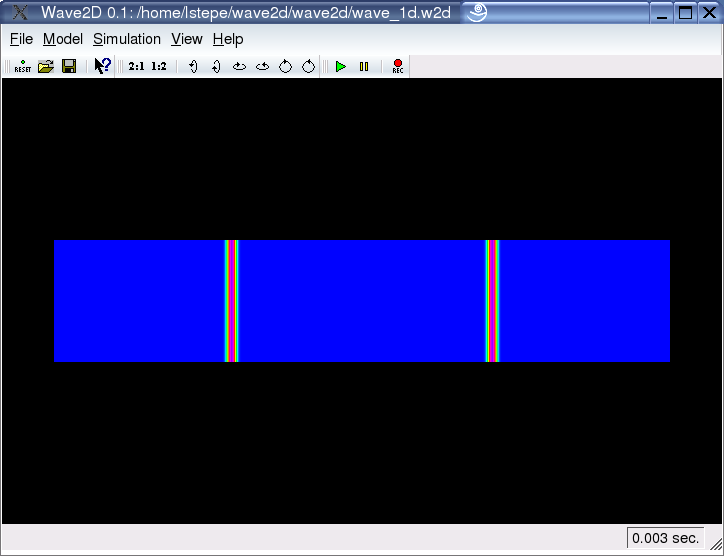
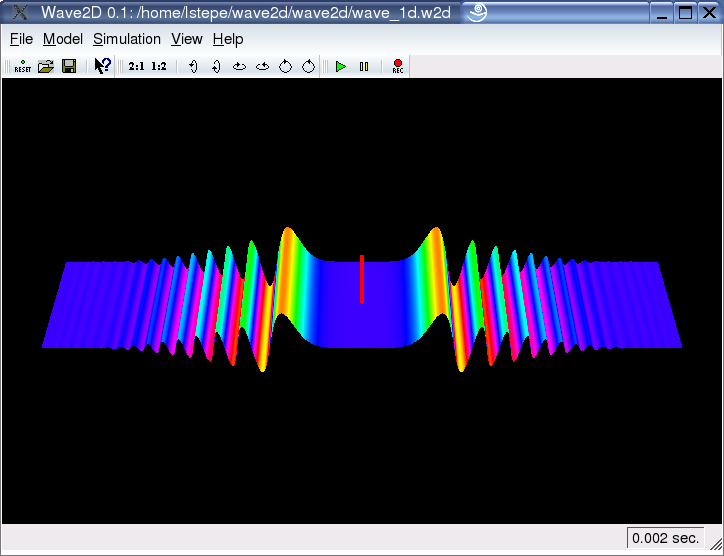
1D Models:
With "Wave2D" it is quite easy to also simulate one-dimensional (1D) models. To do so, one has to take a closer look on the principles of the FTM.
The FTM solves the wave equation by searching for the harmonics of the system. These harmonics are both temporal and spatial eigenmodes of the system. For 2D models these eigenmodes have an order in x1 and an order in x2 dimension. In "Wave2D" one can define maximum values for these "orders". By setting the order in one dimension to 1, one can simply model 1D wave propagation. The pure wave equation can be seen on the left screenshot, the right one shows a metallic model with dispersion, i.e. resistance against bending.
|
|
|
|
|


